Tutorial 2: Fields and Operators
This tutorials covers the basics of setting up and interacting with field and operator objects in Dedalus.
First, we’ll import the public interface and suppress some of the logging messages:
In [1]:
from dedalus import public as de
import numpy as np
import matplotlib.pyplot as plt

de.logging_setup.rootlogger.setLevel('ERROR')
%matplotlib inline
2.1: Fields
Creating a field
Field objects represent scalar fields defined over a domain. A field can
be directly instantiated from the Field class by passing a domain
object, or using the domain.new_field method. Let’s set up a 2D
domain and build a field:
In [2]:
xbasis = de.Fourier('x', 64, interval=(0,2*np.pi), dealias=3/2)
ybasis = de.Chebyshev('y', 64, interval=(-1,1), dealias=3/2)
domain = de.Domain([xbasis, ybasis], grid_dtype=np.float64, mesh=[1])
f = domain.new_field(name='f')
We also gave the field a name – something which is automatically done for the state fields when solving a problem in Dedalus (we’ll see more about this in the next notebook), but we’ve just done it manually, for now.
Manipulating field data
The layout attribute of each field is a reference to the layout
object (discussed in tutorial 1) describing the current
transform/distribution state of that field’s data.
In [3]:
f.layout.grid_space
Out[3]:
array([False, False])
Field data can be written and retrieved in any layout by indexing a
field a layout object. In most cases it’s just the full grid and full
coefficient data that’s most useful to interact with, and these layouts
can be easily accessed using 'g' and 'c' keys as shortcuts.
Field objects also have several methods that can be used to convert the
data between layouts.
Remember that when accessing field data, you’re manipulating just the local data of the globally distributed dataset. Details about the data distribution are available through methods on the layout objects.
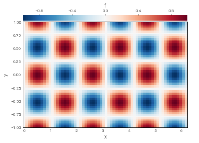
Let’s assign our field some data using the local domain grids.
In [4]:
x, y = domain.grids(scales=1)
# Set data in grid space using 'g' key
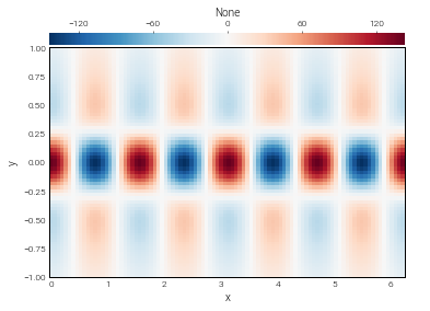
f['g'] = np.cos(4*x) / np.cosh(3*y)
And let’s take a look at this data using some helper functions from the
plot_tools module.
In [5]:
from dedalus.extras.plot_tools import plot_bot_2d
In [6]:
plot_bot_2d(f);
Now let’s take a look at the magnitude of the coefficients:
In [7]:
# Convert data to coefficient space by indexing with 'c' key
f['c']
# Plot log of magnitude of data
def log_magnitude(xmesh, ymesh, data):
    return xmesh, ymesh, np.log10(np.abs(data))
plot_bot_2d(f, func=log_magnitude);
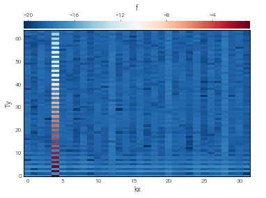
We can see that the specified function is pretty well-resolved.
In addition to the key interface, we can change the layout of a field
using the require_coeff_space, require_grid_space,
require_layout, and require_local methods.
Field scale factors
The set_scales method is used to change the scaling factors used
when transforming field data into grid space. When setting a field’s
data using grid arrays, shape errors will result if there is a mismatch
between the field and grid’s scale factors.
Large scale factors can be used to interpolate the field data onto a high-resolution grid, while small scale factors can be used to view a lower-resolution grid representation of a field. Beware: using scale factors less than 1 will result in a loss of data when transforming to grid space.
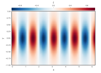
Let’s take a look at a high-resolution sampling of our field, by increasing the scales.
In [8]:
f.set_scales(2)
f['g']
plot_bot_2d(f);
2.2: Operators
Arithmetic with fields
Mathematical operations on fields, such as arithmetic, differentiation,
integration, and interpolation, are represented by operator classes.
An instance of an operator class represents a specific mathematical
operation, and provides an interface for the deferred evaluation of that
operation with respect to it’s potentially evolving arguments.
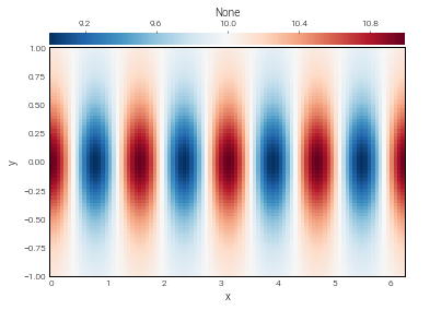
Arithmetic operations between fields, or fields and scalars, are produced simply using Python’s infix operators for arithmetic. Let’s start with a very simple example of adding a scalar to the field we previously defined.
In [9]:
add_op = 10 + f
add_op
Out[9]:
Add(<Scalar 4644516864>, <Field 4603650344>)
The object we get is not another field, but an operator object
representing the addition of 10 and our field. To actually compute this
operation, we use the evaluate method, which returns a new field
with the result. The dealias scale factors set during basis
instantiation are used for the evaluation of all operators.
In [10]:
add_result = add_op.evaluate()
add_result.require_grid_space()
plot_bot_2d(add_result);
Building expressions
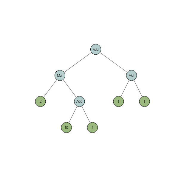
Operator instances can be passed as arguments to other operators, building trees that represent more complicated expressions:
In [11]:
tree_op = 2*add_op + f*f
tree_op
Out[11]:
Add(Mul(<Scalar 4645745944>, Add(<Scalar 4644516864>, <Field 4603650344>)), Mul(<Field 4603650344>, <Field 4603650344>))
Reading these signatures can be a little cumbersome, but we can plot the operator’s structure using a helper from dedalus.tools:
In [12]:
from dedalus.tools.plot_op import plot_operator
plot_operator(tree_op, figsize=8, fontsize=12)
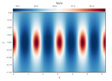
And evaluating it:
In [13]:
tree_result = tree_op.evaluate()
tree_result.require_grid_space
plot_bot_2d(tree_result);
Deferred evaluation
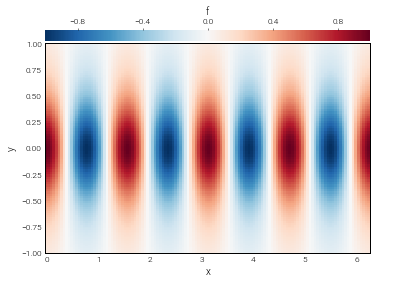
A key point is that the operator objects symbolically represent an operation on the field arguments, and are evaluated using deferred evaluation. If we change the data of the field arguments and re-evaluate an operator, we get a new result.
In [14]:
# Set scales back to 1 to build new grid data
f.set_scales('1', keep_data=False)
f['g'] = np.sin(3*x) * np.cos(6*y)
plot_bot_2d(f);
In [15]:
tree_result = tree_op.evaluate()
tree_result.require_grid_space
plot_bot_2d(tree_result);
Differentiation, integration, interpolation
In addition to arithmetic, operators are used for differentiation, integration, and interpolation. There are three ways to apply these operators to a field.
First, the operators performing these operations along a given dimension
of the data can be accessed through the basis.Differentiate,
basis.Integrate, and basis.Interpolate methods of the
corresponding basis object.
In [16]:
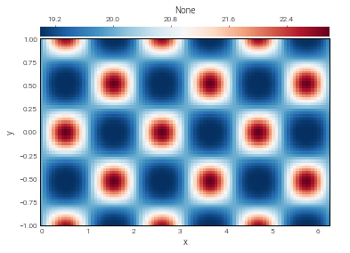
# Let's change the data back to our first example, with a constant offset
f.set_scales('1', keep_data=False)
f['g'] = np.cos(4*x) / np.cosh(3*y) + 1

# Let's setup some operations using the basis operators
fx_op = ybasis.Differentiate(f)
int_f_op = ybasis.Integrate(f)
f0_op = ybasis.Interpolate(f, position=0)

# And we'll just evaluate and plot one of them
fx = fx_op.evaluate()
fx.require_grid_space()
plot_bot_2d(fx);
Second, more general interfaces taking bases as arguments are available
through the operators module. The operators.differentiate
factory allows us to easily construct higher-order and mixed derivatives
involving different bases. The operators.integrate and
operators.interpolate factories allow us to integrate/interpolate
along multiple axes, as well.
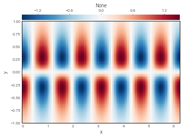
In [17]:
# Some examples using the constructors from the operators module
fxxyy_op = de.operators.differentiate(f, x=2, y=2)
total_int_f_op = de.operators.integrate(f, 'x', 'y')
f00_op = de.operators.interpolate(f, x=0, y=0)

fxxyy = fxxyy_op.evaluate()
total_int_f = total_int_f_op.evaluate()
f00 = f00_op.evaluate()

print('Total integral:', total_int_f['g'][0,0])
print('f at (x,y)=(0,0):', f00['g'][0,0])

fxxyy.require_grid_space()
plot_bot_2d(fxxyy);
Total integral: 12.566370614359172
f at (x,y)=(0,0): 1.9999999999999727

Third, the differentiate, integrate, and interpolate field
methods provide short-cuts for building and evaluating these operations,
directly returning the resulting fields.
In [18]:
# The same results, directly from field methods
fxxyy = f.differentiate(x=2, y=2)
total_int_f = f.integrate('x', 'y')
f00 = f.interpolate(x=0, y=0)

print('Total integral:', total_int_f['g'][0,0])
print('f at (x,y)=(0,0):', f00['g'][0,0])

fxxyy.require_grid_space()
plot_bot_2d(fxxyy);
Total integral: 12.566370614359172
f at (x,y)=(0,0): 1.9999999999999727